K-Nearest Neighbors from scratch
Table of Contents
K-Nearest Neighbors
The K-Nearest Neighbors (KNN) algorithm is a simple and intuitive algorithm that can be used for classification and regression tasks.
In discrete distributions any new data point is given, the algorithm will find the K-nearest neighbors of new points and predict the class of the new point based on the majority vote of the K-nearest neighbors(Generally, K is odd to avoid ties). In case of continuous distributions, the distance between the new point and the K-nearest neighbors is calculated and averaged to get the predicted value. Unlike linear and logistic regression, KNN does not require a linear model to be trained. There are no parameters to be tuned. Its a lazy learning algorithm, the calculations are done at the time of prediction. The distance between the new point and the K-nearest neighbors is calculated using the Euclidean distance. However, other distance metrics can be used as well such as Manhattan distance, Minkowski distance, Cosine distance etc.
What’s the use of KNN
Before we dive into the implementation of KNN, let’s understand the use cases of KNN. When will we ever have dataa bunched by classes and we want to predict the class of new data points? What if we have to predict the preference of a new user based on the preferences of other users? The data of old user is represented as vectors and we can then use KNN to predict whether the new user should be recommanded the product based on KNN.
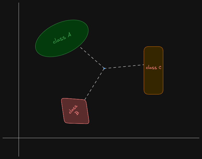
Apart from recommendation, KNN can be used for clustering. For example, if we have a dataset of customers and we want to group them into segments based on their purchase history, we can use KNN to find the K-nearest neighbors of each customer and group them together.
The math behind KNN
The math behind KNN is quite simple compared to other machine learning algorithms.
Euclidian Distance for an ${}n{}$ dimensional vector space is
$$ d = \sqrt{ \sum_{i=1}^n (b_{i}-a_{i})^{2} } $$This simple equation can predict is all that’s needed for KNN.
Implementation
Add the import
import numpy as np
import pandas as pd
import mathplotlib.pyplot as plt
from collections import Counter
from sklearn.model_selection import train_test_split
Load the data and split it into training and testing sets.
data = pd.read_csv('data.csv')
X = data.drop(columns=['id','diagnosis', 'Unnamed: 32']).values
y = data['diagnosis'].values

X_train, X_test, y_train, y_test = train_test_split(X, y, test_size=0.2, random_state=2)
Good ol’ scattar plot
plt.scatter(X_train[y_train=='B',0],X_train[y_train=='B',1],color='tab:green',label='Begin')
plt.scatter(X_train[y_train=='M',0],X_train[y_train=='M',1],color='tab:red',label='Malignant')
plt.xlabel('Radius Mean')
plt.ylabel('Texture Mean')
plt.legend()
plt.show()
Defining Euclidian Distance function
def euclidian_distance(a,b):
  return np.sqrt(np.sum((a-b)**2))
The KNN class is defined as follows
class KNN:
  def __init__(self,k):
    self.k = k
  def fit(self,X,y):
    self.X_train = X
    self.y_train = y
  def predict(self,new_pts):
    predictions = [self.predict_class(new_pt) for new_pt in new_pts]
    return np.array(predictions)
  def predict_class(self,new_pt):
    distances = [euclidian_distance(pt, new_pt) for pt in self.X_train]
    k_nearest_indices = np.argsort(distances)[:self.k]
    k_nearest_labels = [self.y_train[i] for i in k_nearest_indices]
    most_common = Counter(k_nearest_labels).most_common(1)[0][0]
    return most_common
The predict method takes a list of new points and call predict_class for each new point.
Let’s test it out
knn = KNN(11)
knn.fit(X_train,y_train)
predictions = knn.predict(X_test)
accuracy = np.mean(predictions==y_test) * 100
print(f'Accuracy: {accuracy:.2f}%')
Plotting the results
plt.scatter(X_test[predictions=='B',0],X_test[predictions=='B',1],color='tab:green',label='Predicted Begin', marker='x')
plt.scatter(X_test[predictions=='M',0],X_test[predictions=='M',1],color='tab:red',label='Predicted Malignant', marker='x')
plt.xlabel('Radius Mean')
plt.ylabel('Texture Mean')
plt.legend()
plt.show()